The list of the
is a precise description of the randomness in
the system, but the number of quantum states in almost any
industrial system is so high this list is not useable. We thus look
for a single quantity, which is a function of the
, that gives
an appropriate measure of the randomness of a system. As shown
below, the entropy provides this measure.
There are several attributes that the desired function should have.
The first is that the average of the function over all of the
microstates should have an extensive behavior. In other words the
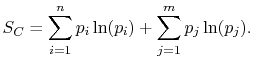
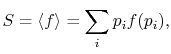
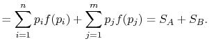
microscopic description of the entropy of a system
, composed of
parts
and
should be given by
![$\displaystyle S_C = S_A+ S_B.$](img907.png) |
(7..4) |
Second is that entropy should increase with randomness and should be
largest for a given energy when all the quantum states are
equiprobable.
The average of the function over all the microstates is defined by
![$\displaystyle S= \langle f\rangle =\sum_i p_i f(p_i),$](img908.png) |
(7..5) |
where the function
is to be found. Suppose that system
has
microstates and system
has
microstates. The
entropies of systems
,
, and
, are defined by
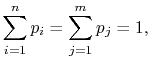
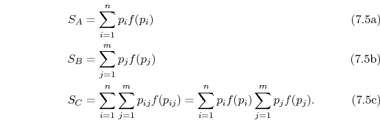
In Equations (7.5) and
(7.6), the term
means the probability
of a microstate in which system
is in state
and system
is in state
. For Equation (7.4) to hold
given the expressions in Equations (7.6),
The function
must be such that this is true regardless of the
values of the probabilities
and
. This will occur if
because
.
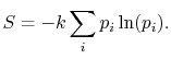
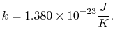
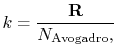
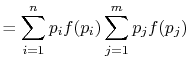
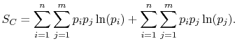
To verify this, make this substitution in the expression for
in the first part of Equation (7.6c)
(assume the probabilities
and
are independent, such that
, and split the log term):
![$\displaystyle S_C=\sum_{i=1}^n\sum_{j=1}^m p_i p_j \ln(p_i)+ \sum_{i=1}^n\sum_{j=1}^m p_i p_j \ln(p_j).$](img922.png) |
(7..8) |
Rearranging the sums, (7.8) becomes
![$\displaystyle S_C = \sum_{i=1}^n\left\{p_i\ln(p_i)\left[\sum_{j=1}^m p_j\right]\right\}+ \sum_{j=1}^m\left\{ p_j\ln(p_j)\left[\sum_{i=1}^n p_i\right]\right\}.$](img923.png) |
(7..9) |
Because
![$\displaystyle \sum_{i=1}^n p_i = \sum_{j=1}^m p_j = 1,$](img924.png) |
(7..10) |
the square brackets in the right hand side of Equation
(7.9) can be set equal to unity, with the result written as
![$\displaystyle S_C=\sum_{i=1}^n p_i\ln(p_i)+\sum_{j=1}^mp_j\ln(p_j).$](img925.png) |
(7..11) |
This reveals the top line of Equation
(7.7) to be the same as the bottom line, for any
,
,
,
, provided that
is a logarithmic function. Reynolds and
Perkins show that the most general
is
,
where
is an arbitrary constant. Because the
are less than
unity, the constant is chosen to be negative to make the entropy
positive.
Based on the above, a statistical definition of entropy can be given
as:
![$\displaystyle S=-k\sum_i p_i \ln(p_i).$](img928.png) |
(7..12) |
The constant
is known as the Boltzmann constant,
![$\displaystyle k =1.380\times10^{-23} \frac{J}{K}.$](img930.png) |
(7..13) |
The value of
is (another wonderful result!) given by
![$\displaystyle k =\frac{\mathbf{R}}{N_\textrm{Avogadro},}$](img931.png) |
(7..14) |
where
is the universal gas constant,
and
is Avogadro's number,
molecules per mol. Sometimes
is called the
gas constant per molecule. With this value for
, the statistical
definition of entropy is identical with the macroscopic definition
of entropy.
UnifiedTP
|